随時更新。だいぶ量が増えてきたので,いくつかを分割したほうが良いかもしれない.
毎回マニュアルから情報を探すのが面倒なので、基本的なものをここにまとめたい。個人的に気になったことに対しては深堀して補足しているが、細かいことを気にしすぎた結果、TikZやPGFのソースコードを読みに行く羽目になった。
またここに書いてある内容がベストプラクティスとは限らないことに注意。もっと簡単な書き方があるかもしれない。
情報の集め方# ここに載っているものはほぼTikZ/PGFのマニュアルに載っている。
この記事では、なるべく参照した情報を記載するようにする。ここに書いてあることが間違っている場合があるので、何かおかしいなと思ったらマニュアルを参照すること。
知らないキーワードや記号が出てきたらマニュアル末尾のindexで探すと良い。 TikZで出来ることを把握したいなら、Part Iのチュートリアルを読んでみるのが有効。もしくはPartIII, Vあたりを流し読みする。PGF Manualはページ数が膨大なため、全部読もうとするのは恐らく得策では無い。目次を眺めながら興味のあるところをつまむのが良いと思う(読み方について、Introductionの1.4 How to Read This Manualも参照)。 既にやりたいことがあるが、TikZで実現する方法が分からない場合は、ググる。英語のキーワードで検索すれば、大抵Stack Exchangeがヒットする。画像検索も有効。 パッケージ読み込み・この記事での記法の注意# TikZはtikzパッケージから読み込める。
以降、コードを記載するときはこの記述を省略する。
また、TikZには色々な便利なライブラリが用意されている。例えば座標計算に便利なライブラリであるCalcは次のように読み込む。
以降、コード中で必要なライブラリがあった場合は、コードの先頭に\usetikzlibraryを記載することにする。
このコマンドは実際にはプリアンブルに書く必要があることに注意。
DVIドライバの指定# 必ずクラスオプションにDVIドライバを指定すること。さもなければ、色が出力されなかったり、図形の位置が正確に計算されなかったりする。
以下は、DVIドライバをdvipdfmx、クラスをjsarticleで行う例。
1
\documentclass [dvipdfmx] { jsarticle}
クラスオプションにDVIドライバを指定する必要性については、以下のサイトを参照:
日本語 LaTeX の新常識 2021 - Qiita 。
色を定義 (TikZの話ではない)# TikZではなくxcolorの話だが、大事なのでここで記す。これはtikzパッケージを読み込んだときに自動で読み込まれるようだが、もしxcolor単体で使いたいなら、xcolorパッケージを読み込むこと。
色同士を!で混ぜることができる。例えばred!20!blue!30!whiteと書くと、赤、青、白がそれぞれ20%、30%、(100-20-30)%混ざった色になる。
カラーコードやRGB値などから定義したい場合は\definecolor、既存の色を混ぜて使いたい場合は\colorletを利用。
1
2
\definecolor { mycolor1}{ HTML}{ 888888} # 定義する色名 カラーモデル 色の値
\colorlet { mycolor2}{ orange!75!white} # 定義する色名 色
色名に-をつけると補色を表現できる。ただし、ここでの補色はRGBでの補色。例えば-redとすると赤色の補色のシアンとなる。RYBでの補色を使いたい場合は-には頼らず、色を直接\definecolorで指定する必要があると思われる。
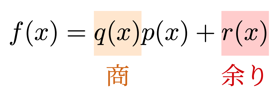
文字にマーカーをつける# 参考 : TikZ で“インラインな”図を描く - Qiita
\tikzはtikzpicture環境がコマンドになっただけで、使い方は同じ。\tikzコマンドのオプション引数baselineで位置を補正。inner sepやouter sepで余白調整。高さを固定したい場合はminimum heightで調整。 枠の下に文字を配置したい場合は、remember pictureとoverlayを利用。
overlayを使わず直接\tikzの中に書いても良いが、文字が多すぎると左右に余計な余白が空く。 1
2
3
4
5
6
7
8
9
10
11
12
13
14
15
16
17
\usetikzlibrary { positioning}
\begin { align*}
f(x) =
\tikz [remember picture, baseline=(T1.base)] {
\node [fill=orange!20!white, inner sep=0pt, outer sep=0, minimum height=4ex] (T1) { $ q ( x ) $ } ;
}
p(x) +
\tikz [remember picture, baseline=(T2.base)] {
\node [fill=red!20!white, inner sep=0pt, outer sep=0, minimum height=4ex] (T2) { $ r ( x ) $ } ;
}
\end { align*}
\begin { tikzpicture} [remember picture, overlay]
\node [below=0pt of T1, text=orange!80!black] { 商} ;
\node [below=0pt of T2, text=red!80!black] { 余り} ;
\end { tikzpicture}
(補足) スタイルを使い回す# スタイルを使いまわしたい場合は、以下の3つの状況において名前/.style={スタイル}のように指定する。
\tikzのオプション引数に指定tikzpicture環境のオプション引数に指定\tikzsetを利用今回は異なる\tikzの間でスタイルを使いまわしたいのでtikzsetが適当。以下のように使う。
1
2
3
4
5
6
7
8
9
10
11
12
\tikzset { box/.style={ inner sep=0pt, outer sep=0, minimum height=4ex}}
\begin { align*}
f(x) =
\tikz [remember picture, baseline=(T1.base)] {
\node [fill=orange!20!white, box] (T1) { $ q ( x ) $ } ;
}
p(x) +
\tikz [remember picture, baseline=(T2.base)] {
\node [fill=red!20!white, box] (T2) { $ r ( x ) $ } ;
}
\end { align*}
なお、styleには引数が指定できる。#1で引数を参照する。スタイルを適用したい要素のオプション引数にて、名前=引数のように使う。2個以上の引数を指定したい場合はstyle n argsを使えばいいらしい。(styleの参考: PGF Manual, Part VII, 87.4.4 Defining Styles)
1
2
3
4
5
6
7
8
9
10
11
12
\tikzset { box/.style={ inner sep=1pt, outer sep=0, minimum height=#1}}
\begin { align*}
f(x) =
\tikz [remember picture, baseline=(T1.base)] {
\node [fill=orange!20!white, box=4ex] (T1) { $ q ( x ) $ } ;
}
p(x) +
\tikz [remember picture, baseline=(T2.base)] {
\node [fill=red!20!white, box=4ex] (T2) { $ r ( x ) $ } ;
}
\end { align*}
Shape# 参考 : PGF Manual, Part V, 71 Shape Library
Shapeライブラリでは色々な図形が定義されている。種類は色々あるのでPDFマニュアル参照。
(補足 Shapeライブラリを使わない方法も後で紹介している。)
shapes.arrowsでsingle arrowとして定義されている。
single arrowで矢印を描画。arrow head extendで矢印の先端の幅を設定。minimum heightで長さ調整。shape border rotate=270で向きを設定。必要に応じてshape border incircleを設定しておく(後述)。1
2
3
4
5
6
7
8
9
\usetikzlibrary { shapes.arrows}
\begin { tikzpicture}
\node at (0, 0) { 命題Pが真} ;
\node [fill=red, single arrow, single arrow head extend=2mm,
minimum height=8mm,
shape border rotate=270] at (0, 1cm) {} ;
\node at (0, 2cm) { 命題Qが真} ;
\end { tikzpicture}
shape border uses incircleは、shapeの境界線がincircle(ノード内のコンテンツを収めるための円。造語?)を使って作られているかどうかを決定するキー。
これを指定すると任意角度の回転ができるようになるが,一方で図形内部にincircleの分スペースが確保されるので,サイズの微調整が少しやりづらくなるかもしれない。
shape border uses incircleを設定しない状態でshape border rotate=aを設定すると、incircle分の余白は空かなくなるが、
代わりにaの部分が「90度の整数倍に最も近い数」に丸められて解釈される。そのため,90度ずつの回転しかできなくなる。
(参考: PGF Manual, Part II, 17.2.3 Common Options)
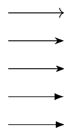
矢印の形を変える# 参考 : PGF Manual, Part III, 16.4.4 Defining Shorthands
終端を変えたいなら>を設定する。他にも色々あるのでマニュアル参照。
1
2
3
4
5
6
7
8
9
\usetikzlibrary { arrows.meta}
\begin { tikzpicture}
\draw [->] (0,0) -- (1,0);
\draw [->, >=Stealth] (0,-0.5) -- (1,-0.5);
\draw [->, >={ Stealth[round]} ] (0,-1.0) -- (1,-1.0);
\draw [->, >=Latex] (0,-1.5) -- (1,-1.5);
\draw [->, >={ Latex[round]} ] (0,-2.0) -- (1,-2.0);
\end { tikzpicture}
巨大な矢印# Shapeライブラリのsingle arrowsを使ってもよいが、以下のようにTriangleの矢印を使うことで同じ図形を再現できる。パラメータは以下の通り。
\drawのline width:線の太さ。\drawのTriangle:outer sepは始点と終点の空白を制御する。詳しくは後述。
1
2
3
4
5
6
7
8
9
10
\usetikzlibrary { arrows.meta}
\begin { tikzpicture}
\node [outer sep=2pt] (p) at (0, 0) { 命題Pが真} ;
\node [outer sep=2pt] (q) at (0, 2cm) { 命題Qが真} ;
\draw [->,
>={ Triangle[width=10mm, length=5mm]} ,
line width=6mm,
red] (q) -- (p);
\end { tikzpicture}
Shapeライブラリの場合は矢印を回転させて使う必要があるが、こちらは向きは自動で変わる。そのため多くの場合はこちらのほうが使いやすいかもしれない。
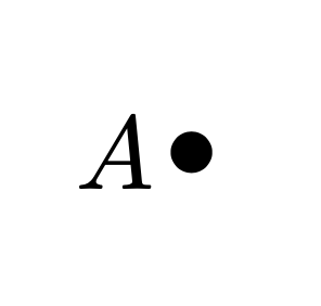
点の上にラベルをつける# 参考 : PGF Manual, Part III, 17.10 The Label and Pin Options
coordinateやnodeにlabelキーを指定すると、例えば図形の点の上にラベルをつけることができる。
例えば以下のようなコードがあったとする。
1
2
3
4
5
6
7
\usetikzlibrary { positioning}
\begin { tikzpicture}
\coordinate (a) at (0,0);
\fill (a) circle [radius=2pt];
\node [left=0pt of a] { $ A $ } ;
\end { tikzpicture}
これが少しだけ簡単になる。
left:を指定しなかった場合はデフォルトでabove:が付く。
1
2
3
4
\begin { tikzpicture}
\coordinate [label=left:$ A $ ] (a) at (0,0);
\fill (a) circle [radius=2pt];
\end { tikzpicture}
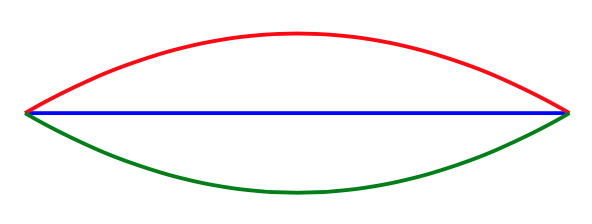
線分を曲げる# 参考 : PGF Manual, Part V, 74 To Path Library
自由に曲線を描きたいなら、\pathのcontrolsを使えば良い(参考: PGF Manual, PartIII, 14.3 The Curve-To Operation)。しかしベジェ曲線に慣れていないと、思い通りの曲線を描くのは大変。しかし、シンプルなケースであればTo Path Libraryを使えば簡単に描ける。
例えば「線分をある方向に曲げたい場合は、bend rightやbend leftが使える。これはTo Path Library で提供されている。以下のようにtoの引数に指定する。
1
2
3
4
5
6
7
8
\begin { tikzpicture}
\coordinate (a) at (0,0);
\coordinate (b) at (2,0);
\draw [blue] (a) -- (b);
\draw [red] (a) to [bend left] (b);
\draw [green!50!black] (a) to [bend right] (b);
\end { tikzpicture}
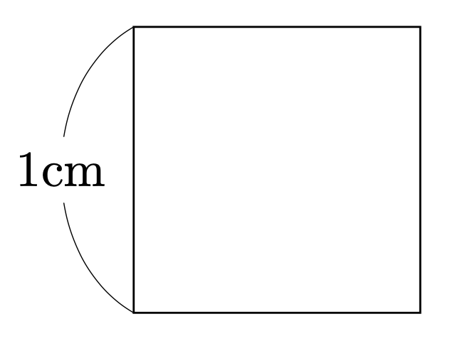
bend right/bend leftは、グラフ構造を描く際に利用できる。また以下のように、図形の長さを明示したいときに使える。
1
2
3
4
5
6
7
8
9
\begin { tikzpicture}
\coordinate (a) at (0,0);
\coordinate (b) at (2,0);
\coordinate (c) at (2,2);
\coordinate (d) at (0,2);
\draw (a) -- (b) -- (c) -- (d) -- cycle;
\draw [line width=0.2pt] (a) to [bend left=60] node [fill=white, midway] { $ 1 $ cm } (d);
\end { tikzpicture}
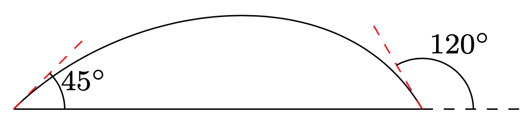
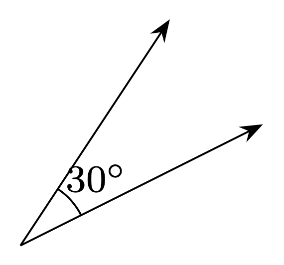
代わりにoutとinを使うと、出ていくときの角度と入っていくときの角度が指定できる。
 1
 2
 3
 4
 5
 6
 7
 8
 9
10
11
12
13
14
15
16
17
18
19
20
21
22
\usetikzlibrary { calc, angles, quotes}
\begin { tikzpicture}
\coordinate (a) at (0,0);
\coordinate (b) at (4,0);
\draw (a) -- (b);
\draw (a) to [out=45, in=120] (b);
% 補助線の描画
\draw [red, dashed] (a) -- ++(45:1cm) coordinate (a1);
\draw [red, dashed] (b) -- ++(120:1cm) coordinate (b1);
\coordinate (a2) at ($ ( a )+( 1 , 0 ) $ );
\coordinate (b2) at ($ ( b )+( 1 , 0 ) $ );
\draw [dashed] (b) -- (b2);
\path pic ["$ 45 ^ \circ $ ", draw, font=\footnotesize , angle eccentricity=1.5]
{ angle=a2--a--a1 } ;
\path pic ["$ 120 ^ \circ $ ", draw, font=\footnotesize , angle eccentricity=1.5]
{ angle=b2--b--b1 } ;
\end { tikzpicture}
bend right/bend leftの初期値# bend leftのデフォルト値はマニュアルによると”(default last value)“と書かれているが、last valueが無い場合の初期値は何なのか不明だったので調べた。ソースコード によると、\tikz@to@bendで定義されているようだ。それはここ で設定されているようで、どうやら30度の模様。
ベクトルや線分# 参考 : PGF Manual, Part III, 13.5 Coordinate Calculations
座標計算にはCalcライブラリが非常に便利。座標同士の足し算や定数倍が行える他、以下で説明する内分点、回転などの計算が行える。
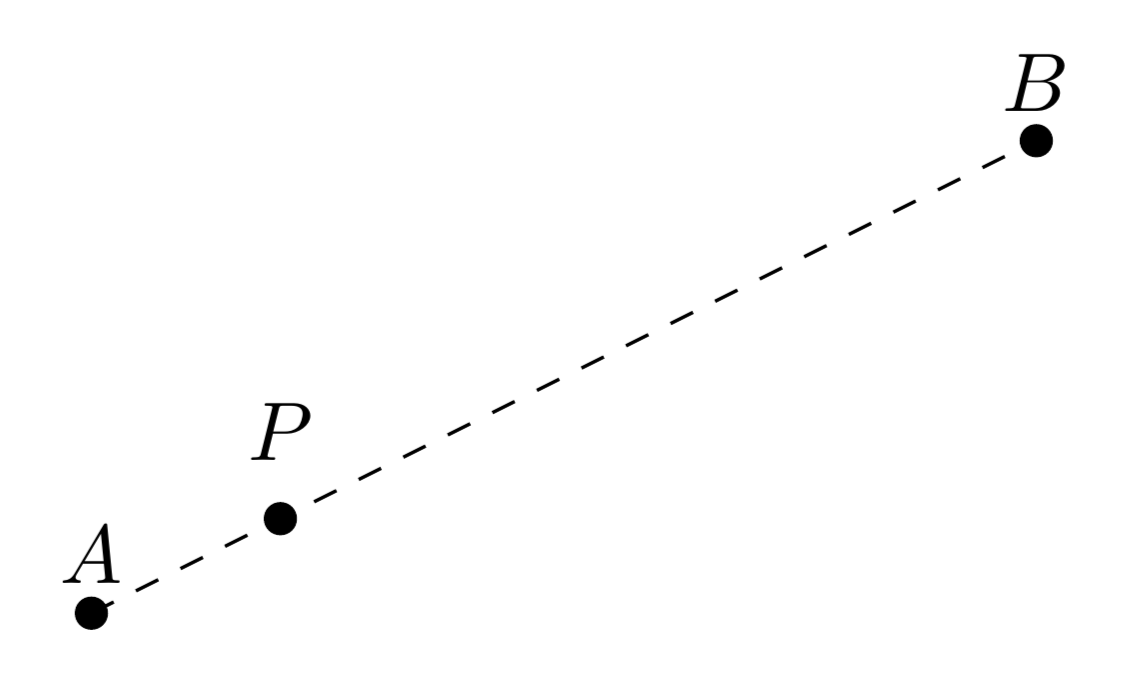
2点間の内分点、外分点# ($(a)!0.2!(b)$)とすると、ab 上の点pで、ap = 0.2ab を満たすものが計算できる。
 1
 2
 3
 4
 5
 6
 7
 8
 9
10
11
12
13
\usetikzlibrary { calc}
\begin { tikzpicture}
\coordinate [label=$ A $ ] (a) at (0,0);
\coordinate [label=$ B $ ] (b) at (4,2);
\fill (a) circle [radius=2pt];
\fill (b) circle [radius=2pt];
\fill ($ ( a )! 0 . 2 !( b ) $ ) node [label=$ P $ ] {} circle [radius=2pt];
\draw [dashed] (a) -- (b);
\end { tikzpicture}
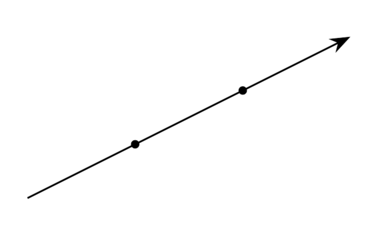
2点間の任意の長さのベクトル# ($(a)!1cm!(b)$)とすると、ab 上の点pで、ap = 1cm を満たすものが計算できる。
1
2
3
4
5
6
7
8
9
10
\usetikzlibrary { calc, arrows.meta}
\begin { tikzpicture}
\coordinate (a) at (0,0);
\coordinate (b) at (2,1);
\draw [->, >=Stealth] (a) -- ($ ( a )! 3 cm !( b ) $ );
\fill ($ ( a )! 2 cm !( b ) $ ) circle [radius=1pt];
\fill ($ ( a )! 1 cm !( b ) $ ) circle [radius=1pt];
\end { tikzpicture}
ベクトルを任意の角度をずらす# ($(a)!1cm!30:(b)$)とすると、「abを30度回転させた線分」 上の点pで、ap = 1cm を満たすものが計算できる。
 1
 2
 3
 4
 5
 6
 7
 8
 9
10
11
12
13
14
15
\usetikzlibrary { calc, angles, quotes, arrows.meta}
\begin { tikzpicture}
\coordinate (a) at (0,0);
\coordinate (t) at (2,1);
\coordinate (b1) at ($ ( a )! 2 cm !( t ) $ );
\coordinate (b2) at ($ ( a )! 2 cm ! 30 : ( t ) $ );
\draw [->, >=Stealth] (a) -- (b1);
\draw [->, >=Stealth] (a) -- (b2);
\path pic ["$ 30 ^ \circ $ ", font=\footnotesize , draw, angle eccentricity=1.5]
{ angle=b1--a--b2 } ;
\end { tikzpicture}
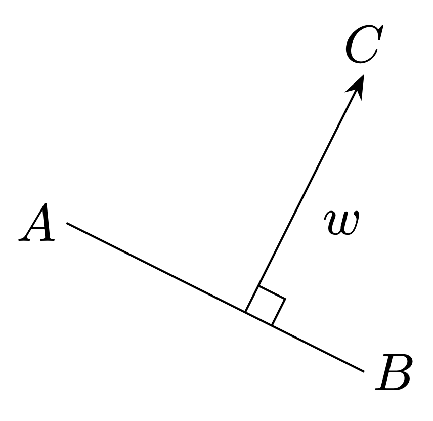
($(a)!(c)!(b)$)とすると、c から ab へ下ろした垂線の足を計算できる。
1
2
3
4
5
6
7
8
9
10
11
12
13
14
15
16
\usetikzlibrary { calc, angles, arrows.meta}
\begin { tikzpicture}
\coordinate (a) at (0,0);
\coordinate (b) at (2,-1);
\coordinate (c) at (2,1);
\coordinate (p) at ($ ( a )!( c )!( b ) $ );
\draw (a) -- (b);
\draw [<-, >=Stealth] (c) -- node [midway, auto] { $ w $ } (p);
\path pic [draw, angle radius=2mm] { right angle=b--p--c } ;
\node [xshift=-2mm] at (a) { $ A $ } ;
\node [xshift=2mm] at (b) { $ B $ } ;
\node [yshift=2mm] at (c) { $ C $ } ;
\end { tikzpicture}
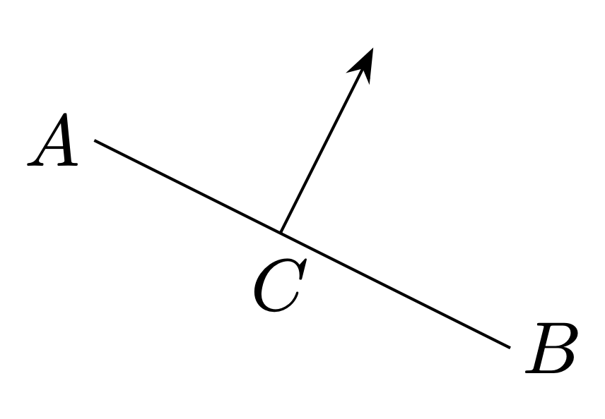
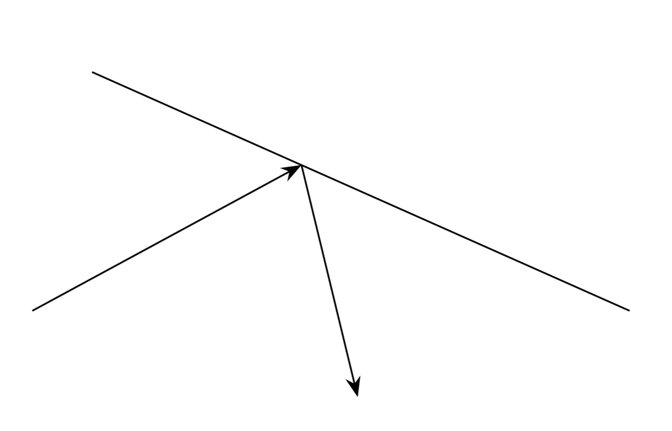
ab 上にある点 c を通る垂線を引きたいなら、線分cbを90度回転させれば良い。
1
2
3
4
5
6
7
8
9
10
11
12
13
14
\usetikzlibrary { calc, arrows.meta}
\begin { tikzpicture}
\coordinate (a) at (0,0);
\coordinate (b) at (2,-1);
\coordinate (c) at ($ ( a )! 1 cm !( b ) $ );
\draw (a) -- (b);
\draw [->, >=Stealth] (c) -- ($ ( c )! 1 cm ! 90 : ( b ) $ );
\node [xshift=-2mm] at (a) { $ A $ } ;
\node [xshift=2mm] at (b) { $ B $ } ;
\node [yshift=-2.5mm] at (c) { $ C $ } ;
\end { tikzpicture}
垂線(縦軸または横軸に対して)# 参考 : PGF Manual, Part III, 13.3.1 Intersections of Perpendicular Lines
前節では垂線を求めるのに3点の座標を使ったが、特別なケースでは2点で垂線を引くことができるので、それを紹介する。
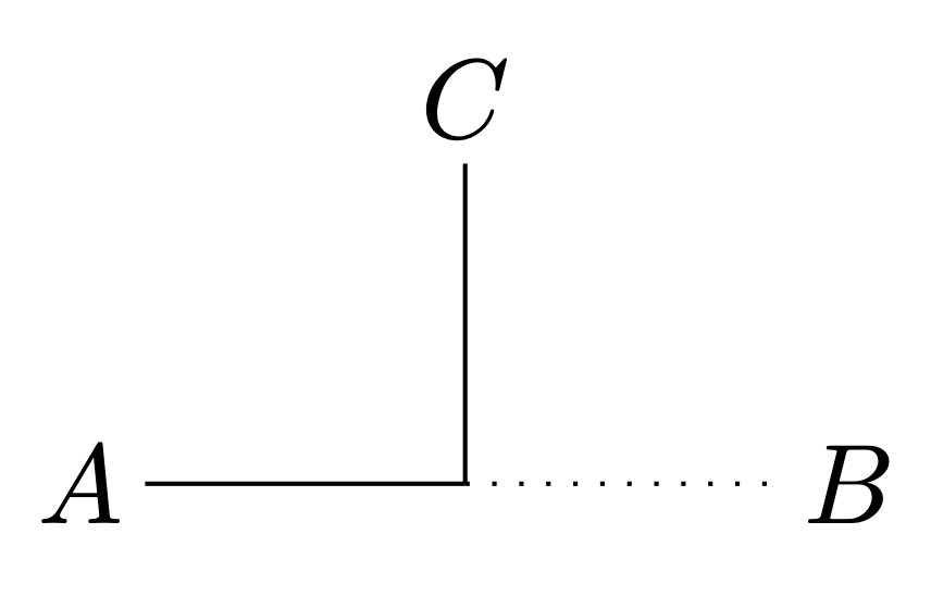
(c |- a)とすると、c から 「aを通る、横軸に平行な直線」との垂線の足を求められる。
前節では垂線の足を求めるためにはbの座標が必要だったが、横軸に平行な場合は必要ない。
ちなみに見方を変えると「cを通る、縦軸に平行な直線」との垂線の足とも捉えられる。
また、(a -| c)のように逆向きに書くことが可能である。
(a |- c)なのか(c |- a)なのか混乱するかもしれないが、その都度実際に描画してみて確認すれば良いと思う。
 1
 2
 3
 4
 5
 6
 7
 8
 9
10
11
12
13
14
\begin { tikzpicture}
\coordinate (a) at (0,0);
\coordinate (b) at (2,0);
\coordinate (c) at (1, 1);
\coordinate (p) at (c |- a);
\draw (a) -- (p);
\draw [dotted] (p) -- (b);
\draw (c) -- (p);
\node [xshift=-2mm] at (a) { $ A $ } ;
\node [xshift=2mm] at (b) { $ B $ } ;
\node [yshift=2mm] at (c) { $ C $ } ;
\end { tikzpicture}
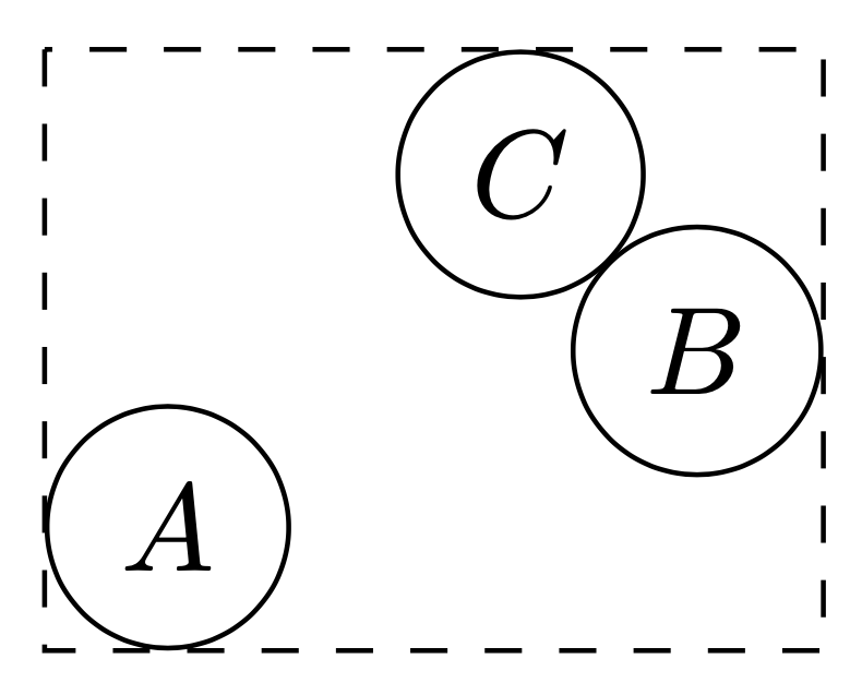
垂線の足としての使い方だけでなく、「2点A, Cを始点として横軸方向、縦軸方向にそれぞれ伸ばし、ぶつかった点を計算する」という用途で使うこともある。例えば、以下は黒枠でノードを囲む例である(実は Fitting Library を使うともっと直感的に書ける)。
1
2
3
4
5
6
\begin { tikzpicture} [every node/.style={ draw, circle} ]
\node (a) at (0,0) { $ A $ } ;
\node (b) at (1.5,0.5) { $ B $ } ;
\node (c) at (1,1) { $ C $ } ;
\draw [dashed] (c.north -| a.west) rectangle (a.south -| b.east);
\end { tikzpicture}
ベクトルを平行にずらす# xy軸ごとの移動方向vが決まっているなら、$(a) + (v)$みたいに計算するか、、scope環境でくくってxshiftとyshiftを使えば良い(参考 : PGF Manual, Part III, 25.3 Coordinate Transformations)。
もし「ベクトルabを平行移動したいが、移動の向きはabの法線方向にしたい」という場合は、次のように c、d を計算する。
($(a)!1cm!90:(b)$)については以前説明した通り。($(b)+(c)-(a)$)で、「点bをベクトルacだけ移動した点」を計算している。
1
2
3
4
5
6
7
8
9
10
11
12
\usetikzlibrary { calc, arrows.meta}
\begin { tikzpicture}
\coordinate (a) at (0,0);
\coordinate (t) at (4,2);
\coordinate (b) at ($ ( a )! 1 cm !( t ) $ );
\draw (a) -- (t);
\coordinate (c) at ($ ( a )! 0 . 2 cm ! 90 : ( b ) $ );
\coordinate (d) at ($ ( b )+( c )-( a ) $ );
\draw [->, >=Stealth, thick, red] (c) -- node [midway, auto] { $ v $ } (d);
\end { tikzpicture}
座標計算のネスト# 座標の計算は($...$)で行うが、これはネストすることができる。
例えば、点aとbに対して、2(b-a)のようなベクトルを計算したい場合は、
($2*($(b) - (a)$)$)のように計算する。もし($2*((b) - (a))$)みたいに計算できたら直感的で良かったのだが、Calcライブラリのシンタックスの都合上($...$)をネストさせないといけない。
(細かい話)Calcライブラリのシンタックスについて# シンタックスについて少し説明する。
まず、“PGF Manual Part III, 13.5.1 The General Syntax"によると、
一般のシンタックスは([<options>]$<coordinate computation>$)。 <coordinate computation>は、<factor>*<coordinate><modifiers>で始まる。任意で +または-が続き、その後に<factor>*<coordinate><modifiers>が続く。 同様にして、+または-が続き、そのあとに上記の<factor>...が続く。 と書かれている。ただし、[<options>]、<factor>*、<modifiers>はそれぞれ、
[<options>]:何らかのオプションを設定する(Calcライブラリの場合、これが果たして何に使われるのか不明)。<factor>*:スカラー倍。例えば2*(a)の2*の部分。<modifiers>:前述の、2点間の内分点外分点 、2点間の任意の長さのベクトル のためのシンタックス。例えば(a)!0.5!(b)の!0.5(b)の部分。詳しい文法は"13.5.3 The Syntax of Partway Modifiers"や"13.5.4 The Syntax of Distance Modifiers"を参照。を意味する。これらは省略可能である。
上記より、Calcライブラリで行う計算のシンタックスをBNF風に書くと以下のようになってるらしいことが分かる(合っているか少し不安だが)。
1
2
3
4
5
<coordinate> := ([<options>]$⟨coordinate computation⟩$)
<coorinate computation> := <modified coordinate>
| <modified coordinate> + <modified coordinate>
| <modified coordinate> - <modified coordinate>
<modified coordinate> := <factor>*<coordinate><modifiers>
ただし、[<options>]、<factor>、<modifiers>をつけるかは任意である。
また、<coordinate>として、TikZ標準の(a)や(1, 2)、(5mm, 1mm)などの表記もあり得るが、ここでは省略している。
上のBNF風の表現に照らし合わせると、
という計算はシンタックスエラーになることが分かる。
なぜなら、内側の2*((b) - (a))は<factor>*<coordinate><modifiers>の形であり、
((b) - (a))は<coordinate>の定義に反しているからである。
($(b) - (a))$なら<coordinate>の定義に沿っている。
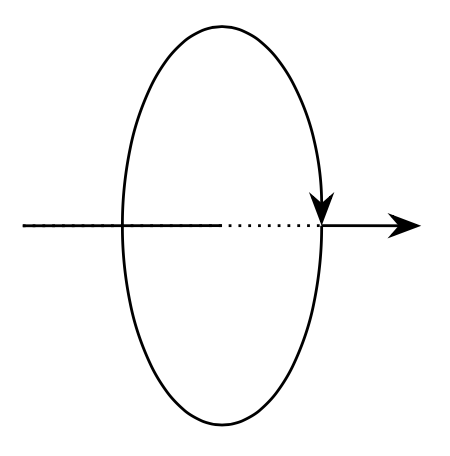
交点の計算# 参考 PFG Manual, Part III, 13.3.2 Intersections of Arbitrary Paths
name pathでパスの名前を指定して、name intersectionsでパス同士の交点を計算する。
name intersectionsについて、ofに2つのパス名を指定する。
byには交点の名前を指定する。円と線分には2つの交点があるので、byに2つの名前を指定している。
1
2
3
4
5
6
7
8
9
10
11
12
13
14
15
16
17
\usetikzlibrary { intersections}
\begin { tikzpicture} [>=Stealth, arrows.meta]
\coordinate (e1) at (-1, 0);
\coordinate (e2) at (1, 0);
\path [name path=circle1] circle [x radius=0.5cm, y radius=1cm];
\path [name path=line1] (e1) -- (e2);
\path [name intersections={ of=circle1 and line1, by={ b,a}} ];
\coordinate (c) at ($ ( a )! 0 . 5 !( b ) $ );
\draw [->] (0.5cm, 0) arc [start angle=0, end angle=-360, x radius=0.5cm, y radius=1cm];
\draw (e1) -- (c);
\draw [densely dotted] (e1) -- (b);
\draw [->] (b) -- (e2);
\end { tikzpicture}
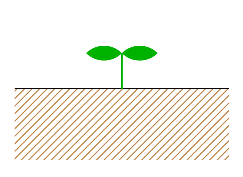
斜線で領域を塗る# 参考 : PGF Manual, Part V, 62 Pattern Library
Patternsライブラリを使えば良い。patternで使いたいパターンを指定し、pattern colorで色を設定。
1
2
3
4
5
6
7
8
9
\usetikzlibrary { patterns}
\begin { tikzpicture}
\draw (0,0) -- (3,0);
\draw [green!70!black, thick] (1.5,0) -- (1.5,0.5);
\fill [green!70!black] (1.5,0.5) to [bend left=45] (2.0,0.5) to [bend left=45] cycle;
\fill [green!70!black] (1.5,0.5) to [bend right=45] (1.0,0.5) to [bend right=45] cycle;
\path [pattern=north east lines, pattern color=brown] (0,0) rectangle (3, -1);
\end { tikzpicture}
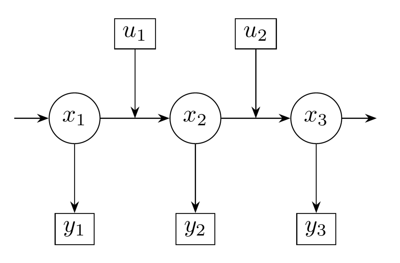
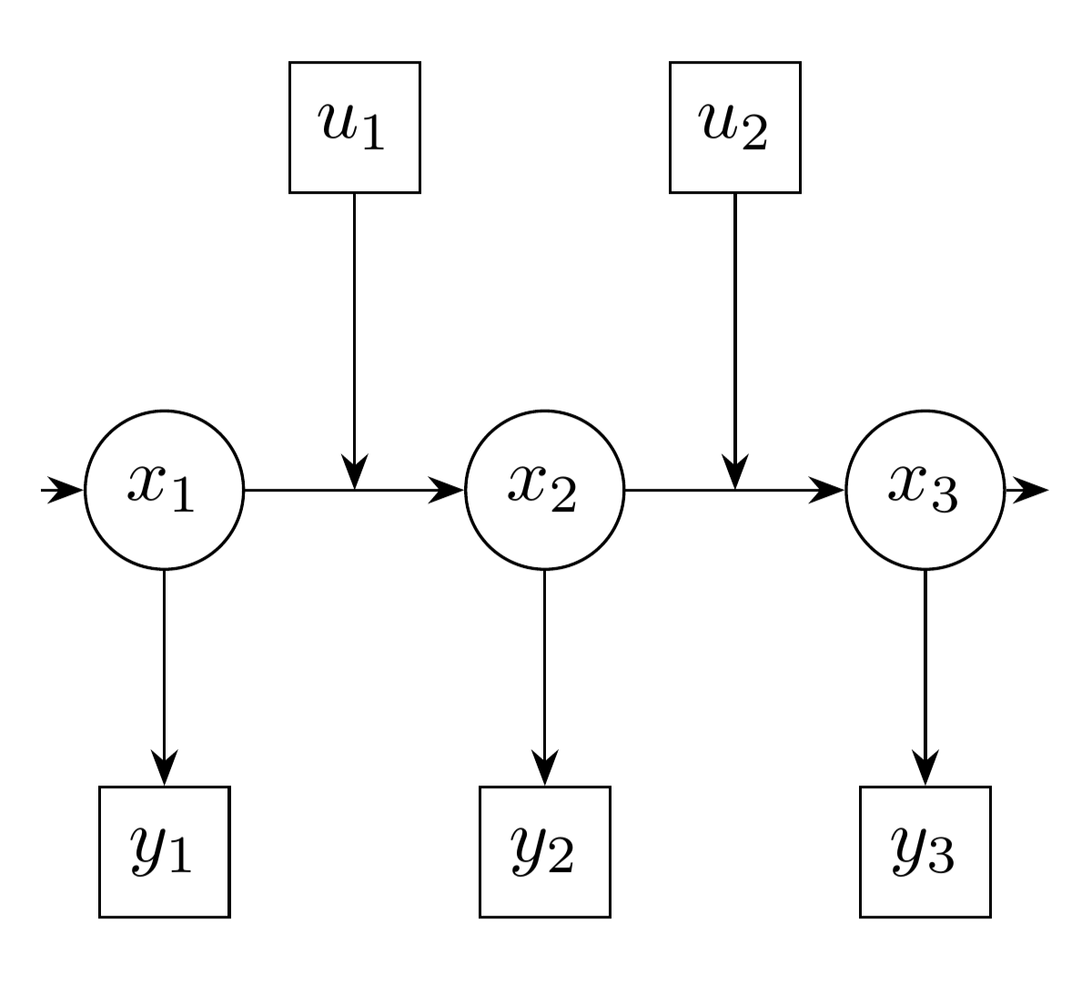
並べる方法# 相対位置で指定する# 参考
PGF Manual, Prat III, 17.5.3 Advanced Placement Options PGF Manual, Part III, 19 Specifying Graphs 位置の指定には、right=1cm of (a)だったり、($(a)!0.5!(b)$)を利用。
graphを使うと、グラフがより簡潔に書ける。\draw [->] (x1) -- (x2);みたいに矢印を1つずつ描かず、
直感的な記述でノード間の関係を記述できる。
\graphのedgesパラメータで、グラフ内の辺のスタイルを設定できる。
 1
 2
 3
 4
 5
 6
 7
 8
 9
10
11
12
13
14
15
16
17
18
19
20
21
22
23
24
25
26
27
28
29
30
31
\usetikzlibrary { calc, positioning, graphs, arrows.meta}
\begin { tikzpicture}
[entity-x/.style={ draw, circle} ,
entity-u/.style={ draw} ,
entity-y/.style={ draw} ]
\node [entity-x] (x1) { $ x_ 1 $ } ;
\node [right=1cm of x1, entity-x] (x2) { $ x_ 2 $ } ;
\node [right=1cm of x2, entity-x] (x3) { $ x_ 3 $ } ;
\coordinate (x0) at ($ ( x 1 )-( 1 , 0 ) $ );
\coordinate (x4) at ($ ( x 3 )+( 1 , 0 ) $ );
\coordinate (x1-2) at ($ ( x 1 )! 0 . 5 !( x 2 ) $ );
\coordinate (x2-3) at ($ ( x 2 )! 0 . 5 !( x 3 ) $ );
\node [above=1cm of x1-2, entity-u] (u1) { $ u_ 1 $ } ;
\node [above=1cm of x2-3, entity-u] (u2) { $ u_ 2 $ } ;
\node [below=1cm of x1, entity-y] (y1) { $ y_ 1 $ } ;
\node [below=1cm of x2, entity-y] (y2) { $ y_ 2 $ } ;
\node [below=1cm of x3, entity-y] (y3) { $ y_ 3 $ } ;
\graph [edges={ >=Stealth} ]{
(x0) -> (x1) -> (x2) -> (x3) -> (x4);
(u1) -> (x1-2);
(u2) -> (x2-3);
(x1) -> (y1);
(x2) -> (y2);
(x3) -> (y3);
} ;
\end { tikzpicture}
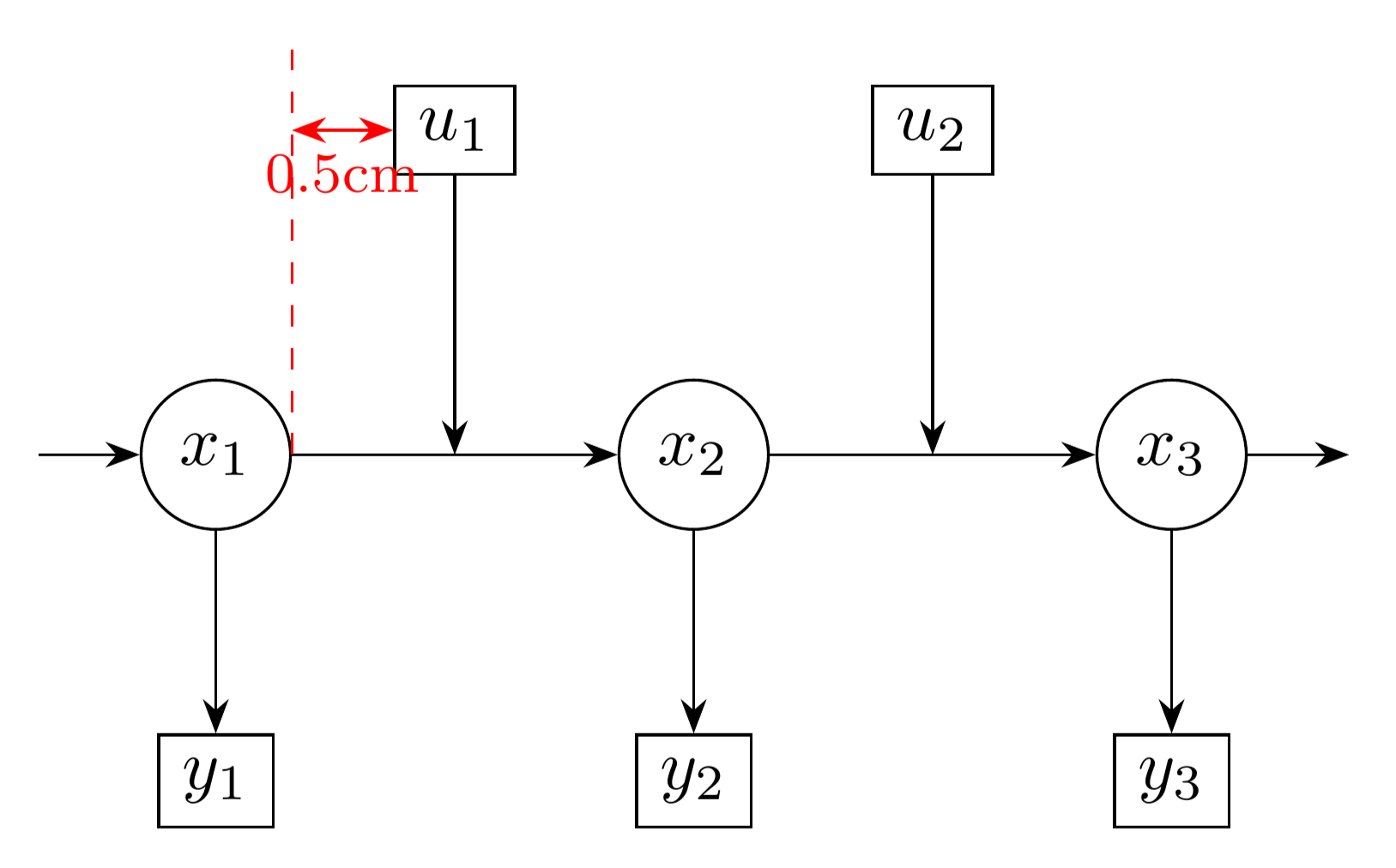
matrixで指定する# 参考 : PGF Manual, Part III, 20 Matrices and Alignment
\matrixを使うと、図形やノードを格子上に並べることができる。
row sepやcolumn sepの指定に注意 (図の赤文字を参考)。
 1
 2
 3
 4
 5
 6
 7
 8
 9
10
11
12
13
14
15
16
17
18
19
20
21
22
23
24
25
26
27
28
29
30
\usetikzlibrary { graphs, arrows.meta}
\begin { tikzpicture}
[entity-x/.style={ draw, circle} ,
entity-u/.style={ draw} ,
entity-y/.style={ draw} ,
>=Stealth]
\matrix [row sep=1cm, column sep=0.5cm] {
& & \node [entity-u] (u1) { $ u_ 1 $ } ; & & \node [entity-u] (u2) { $ u_ 2 $ } ; & & \\
\coordinate (x0) at (0,0); & \node [entity-x] (x1) { $ x_ 1 $ } ; &
\coordinate (x1-2) at (0,0); & \node [entity-x] (x2) { $ x_ 2 $ } ; &
\coordinate (x2-3) at (0,0); & \node [entity-x] (x3) { $ x_ 3 $ } ; &
\coordinate (x4) at (0,0);\\
& \node [entity-y] (y1) { $ y_ 1 $ } ; & & \node [entity-y] (y2) { $ y_ 2 $ } ; & & \node [entity-y] (y3) { $ y_ 3 $ } ; & \\
} ;
\graph {
(x0) -> (x1) -> (x2) -> (x3) -> (x4);
(u1) -> (x1-2);
(u2) -> (x2-3);
(x1) -> (y1);
(x2) -> (y2);
(x3) -> (y3);
} ;
\coordinate (a) at ($ ( x 1 .east ) + ( 0 , 2 cm ) $ );
\draw [red, dashed] (x1.east) -- (a);
\draw [red, <->] (u1.west) -- node [midway, auto, font=\footnotesize ] { $ 0 . 5 $ cm } ($ ( x 1 .east )!( u 1 .west )!( a ) $ );
\end { tikzpicture}
node関連# 参考 : PGF Manual, Part III, 17.2.3 Common Options: Separations, Margins, Padding and Border Rotation
サイズ変更# minimum width、minimum heightを使う。ノード同士のサイズを合わせたいならこれを使うとよい。
 1
 2
 3
 4
 5
 6
 7
 8
 9
10
11
12
13
14
15
16
17
18
19
20
21
22
23
24
25
26
\usetikzlibrary { graphs, arrows.meta}
\begin { tikzpicture}
[entity-x/.style={ draw, circle, minimum height=4ex} ,
entity-u/.style={ draw, minimum width=4ex, minimum height=4ex} ,
entity-y/.style={ draw, minimum width=4ex, minimum height=4ex} ,
>=Stealth]
\matrix [row sep=1cm, column sep=0.2cm] {
& & \node [entity-u] (u1) { $ u_ 1 $ } ; & & \node [entity-u] (u2) { $ u_ 2 $ } ; & & \\
\coordinate (x0) at (0,0); & \node [entity-x] (x1) { $ x_ 1 $ } ; &
\coordinate (x1-2) at (0,0); & \node [entity-x] (x2) { $ x_ 2 $ } ; &
\coordinate (x2-3) at (0,0); & \node [entity-x] (x3) { $ x_ 3 $ } ; &
\coordinate (x4) at (0,0);\\
& \node [entity-y] (y1) { $ y_ 1 $ } ; & & \node [entity-y] (y2) { $ y_ 2 $ } ; & & \node [entity-y] (y3) { $ y_ 3 $ } ; & \\
} ;
\graph {
(x0) -> (x1) -> (x2) -> (x3) -> (x4);
(u1) -> (x1-2);
(u2) -> (x2-3);
(x1) -> (y1);
(x2) -> (y2);
(x3) -> (y3);
} ;
\end { tikzpicture}
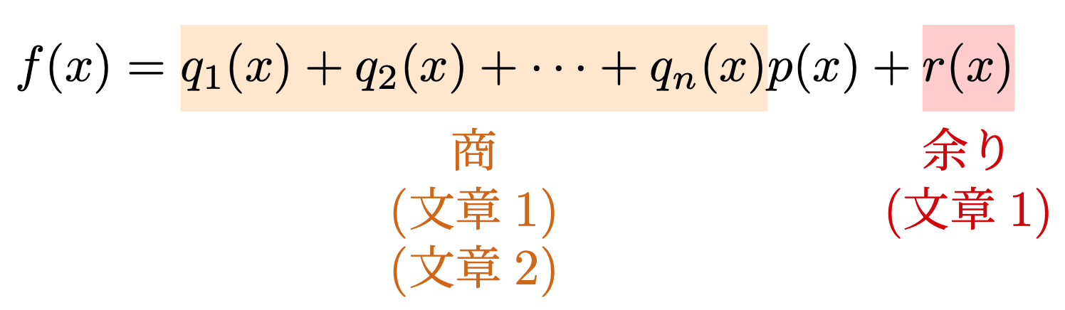
改行できるようにする# nodeのオプション引数にalignを設定する。center、left、rightなどが指定できる。
 1
 2
 3
 4
 5
 6
 7
 8
 9
10
11
12
13
14
15
16
17
18
19
20
21
22
23
24
\usetikzlibrary { positioning}
\begin { align*}
f(x) =
\tikz [remember picture, baseline=(T1.base)] {
\node [fill=orange!20!white, box=4ex] (T1) { $ q_ 1 ( x ) + q_ 2 ( x ) + \cdots + q_n ( x ) $ } ;
}
p(x) +
\tikz [remember picture, baseline=(T2.base)] {
\node [fill=red!20!white, box=4ex] (T2) { $ r ( x ) $ } ;
}
\end { align*}
\begin { tikzpicture} [remember picture, overlay]
\node [below=0pt of T1, text=orange!80!black, align=center]
{ 商\\ [-1ex]
(文章1)\\ [-1ex]
(文章2)\\ [-1ex]
} ;
\node [below=0pt of T2, text=red!80!black, align=center]
{ 余り\\ [-1ex]
(文章1)\\ [-1ex]
} ;
\end { tikzpicture}
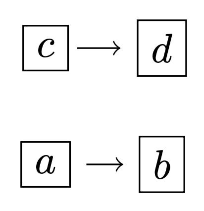
矢印とノードとの余白を空ける# 手軽な方法として2つ思い浮かんだ。1つ目は、node側でouter sepを指定する方法。始点と終点の余白を同じにしたいならこちらの方法が簡潔。2つ目は、draw側でshorten <とshorten >を指定する方法。それぞれ始点と終点の長さを指定できるため自由度が高い。
1
2
3
4
5
6
7
8
9
\begin { tikzpicture}
\node [draw, outer sep=4pt] (a) at (0,0) { $ a $ } ;
\node [draw, outer sep=4pt] (b) at (1,0) { $ b $ } ;
\node [draw] (c) at (0,1) { $ c $ } ;
\node [draw] (d) at (1,1) { $ d $ } ;
\draw [->] (a) -- (b);
\draw [->, shorten <=2pt, shorten >=4pt] (c) -- (d);
\end { tikzpicture}
繰り返し文# 参考 : PGF Manual, Part VII, 88 Repeating Things: The Foreach Statement
\foreachが用意されている。{0.5,1,...,3}のように、規則性を持つリストは...で省略できる場合がある。
1
2
3
4
5
6
\begin { tikzpicture}
\draw circle [radius=0.25];
\foreach \r in { 0.5,1,...,3} {
\draw [orange, thick] (80:\r ) arc [radius=\r , start angle=80, delta angle=-60];
}
\end { tikzpicture}
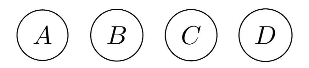
C言語のifやfor文みたいに、繰り返したい対象が1文の場合はブロック{}で括らなくても良い。
また、複数のパラメータを/で区切って使用できる。
1
2
3
4
\begin { tikzpicture}
\foreach \x /\l in { 1/A, 2/B, 3/C, 4/D}
\node [draw, circle] at (\x , 0) { $ \l $ } ;
\end { tikzpicture}
関数を使う# 参考 : PGF Manual, Part VIII, 94 Mathematical Expressions
これはTikZの話というより、TikZが内部で利用しているPGFの話になる。
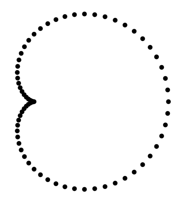
cosやsinなどの基本的な関数が使える。関数を評価したいときは{}で囲む。
1
2
3
4
5
\begin { tikzpicture}
\foreach \theta in { 0,5,10,...,359}
\fill ({ (1+cos(\theta ))*cos(\theta )} , { (1+cos(\theta ))*sin(\theta )} )
circle [radius=1pt];
\end { tikzpicture}
関数以外にも色々な2項演算子や定数が用意されているようなので、マニュアルを見てみると良い。
array-likeなデータ構造も用意されているらしい。
(込み入った補足) 波括弧(curly braces)について# 以下のような、関数を使わない場合は波括弧をつけなくても良いようだ。
1
2
3
\begin { tikzpicture}
\fill (1+2, 3) circle [radius=1pt];
\end { tikzpicture}
もちろん波括弧をつけても良い。
1
2
3
\begin { tikzpicture}
\fill ({ 1+2} , 3) circle [radius=1pt];
\end { tikzpicture}
しかし、マニュアルでは波括弧はarray-likeなオブジェクトを表す記号のはず。内部では1+2も{1+2}もともに3と評価されているようだ。この理由が気になる。
まず波括弧の処理がどこで行われているのかを探す。TikZの計算で例外的に波括弧が処理されるのか、それとも\pgfmathparseで処理されるのか。
まずTikZのソースコードを覗いてみる。
色々探してみたところ、canvas座標系での計算は
ここ
でやっているようだ。
1
2
3
4
5
\tikzdeclarecoordinatesystem { canvas}
{ %
\tikzset { cs/.cd,x=0pt,y=0pt,#1} %
\pgfpoint { \tikz @cs@x}{ \tikz @cs@y} %
} %
座標の計算はここでは行わず、\pgfpointに頼っている。そこでpgfpointのソースコード を見に行く。
1
2
3
\def\pgfpoint #1#2{ %
\pgfmathsetlength\pgf @x{ #1} %
\pgfmathsetlength\pgf @y{ #2} \ignorespaces }
\pgf@x、\pgf@yというのは、xy座標を入れるためのレジスタだと予想できる。続いて、pgfmathsetlengthのソースコード を見にいく。
1
2
3
4
5
6
7
8
9
10
11
\def\pgfmathsetlength #1#2{ %
\expandafter\pgfmath @onquick#2\pgfmath @%
{ %
% ...略
} %
{ %
\pgfmathparse { #2} %
% ...略
} %
\ignorespaces %
}
このタイミングで\pgfmathparseが呼び出されているようだ。\pgfmathparseで式を評価し、\pgfmathresultで評価結果を取得しているようである。
結局、波括弧をつけるか否かは\pgfmathparse及びその結果である\pgfmathresultに委ねられているようだ。\pgfmathparseのコードを読む気力がなかったので、\showマクロで展開結果を見てみる。
1
2
3
4
5
6
7
8
9
10
11
% 数字のパース
\pgfmathparse { 1}
\show\pgfmathresult
% 波括弧で括られた数字のパース
\pgfmathparse {{ 1}}
\show\pgfmathresult
% array-likeなオブジェクトのパース
\pgfmathparse {{ 1,2,3}}
\show\pgfmathresult
これでタイプセットしてみる。
> \pgfmathresult=macro:
->1.
l.280 \show\pgfmathresult
?
> \pgfmathresult=macro:
->1.
l.283 \show\pgfmathresult
?
> \pgfmathresult=macro:
->{1}{2}{3}.
l.286 \show\pgfmathresult
初めの2つは1と展開され、最後の1つは{1}{2}{3}と展開された。
どうやら波括弧の要素が1つの場合は結果が波括弧で包まれないらしい。
ただし、以下の計算はエラーになるので、{1}はarray-likeではあるようだ。
x座標、y座標を個別に取得# 参考 : PGF Manual, Part III, 14.15 The Let Operation
letを使う。letを使うと、座標や値を入れるレジスタが作成できる。
以下は、反射角の計算のためにletを使っている。\p<name>、\n<name>は特殊なレジスタ。前者は点の座標を保持し、\x<name>、\y<name>で点の座標にアクセスできる。後者は値を保持し、\n<name>でアクセスできる。<name>の部分には、数字や{文字列}が指定できる例えば\p1、\p{foo}のように使う。
 1
 2
 3
 4
 5
 6
 7
 8
 9
10
11
12
13
14
15
16
17
18
19
\usetikzlibrary { calc, arrows.meta}
\begin { tikzpicture} [>=Stealth]
\coordinate (a) at (0.5, 2);
\coordinate (b) at (5, 0);
\coordinate (o) at (0,0);
\draw [name path=line1] (a) -- (b);
\path [name path=line2] (o) -- (1cm:15);
\path [name intersections={ of=line1 and line2, by={ p}} ];
\draw [->] (o) -- (p);
\draw [->]
let \p 1 = ($ ( a ) - ( p ) $ ),
\p 2 = ($ ( o ) - ( p ) $ ),
\n 1 = { atan2(\y 2, \x 2)-atan2(\y 1, \x 1)}
in
(p) -- ($ ( p )! 2 cm !- \n 1 : ( b ) $ );
\end { tikzpicture}
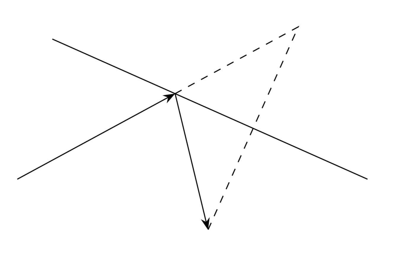
座標計算を行いたい多くの場合は、letを使わなくても解決できる気がする。例えば反射の場合は、一旦延長してから垂線を伸ばせば良い。
 1
 2
 3
 4
 5
 6
 7
 8
 9
10
11
12
13
14
15
16
17
18
19
\usetikzlibrary { calc, arrows.meta}
\begin { tikzpicture} [>=Stealth]
\coordinate (a) at (0.5, 2);
\coordinate (b) at (5, 0);
\coordinate (o) at (0,0);
\draw [name path=line1] (a) -- (b);
\path [name path=line2] (o) -- ++(1cm:15);
\path [name intersections={ of=line1 and line2, by={ p}} ];
\coordinate (q) at ($ ( p ) + ( o )! 2 cm !( p ) $ );
\coordinate (r) at ($ ( a )!( q )!( b ) $ );
\coordinate (s) at ($ ( q )! 2 !( r ) $ );
\draw [->] (o) -- (p);
\draw [dashed] (p) -- (q) -- (s);
\draw [->] (p) -- (s);
\end { tikzpicture}
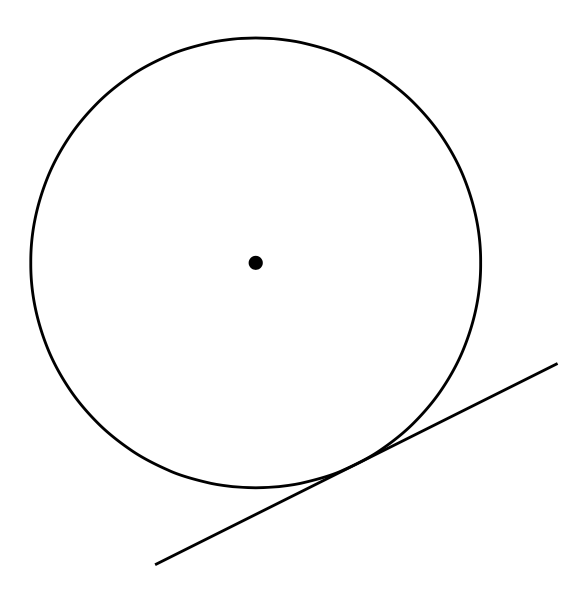
PGF Manualでは「直線に接する円」を描画するためにletを使っていた。例えば半径のような、座標以外の計算をしたい場合にlet式が有効なのだと思う。
1
2
3
4
5
6
7
8
9
10
11
12
\usetikzlibrary { calc}
\begin { tikzpicture}
\coordinate (a) at (0,0);
\coordinate (b) at (2,1);
\coordinate (c) at (0.5,1.5);
\draw (a) -- (b);
\fill (c) circle [radius=1pt];
\draw let \p 1 = ($ ( a )!( c )!( b ) - ( c ) $ )
in
(c) circle [radius={ veclen(\x 1,\y 1)} ];
\end { tikzpicture}
レイヤを使う# 参考 PGF Manual, Part IX, 113 Layered Graphics
描画順を制御したいときがたまにある。そんなときはレイヤの仕組みを使う。
TikZコマンドは、基本的に書いた順に実行され、図形が重ねられる。
そのため、描画順を変えたいなら、素朴にはTikZコマンドの順番を変えれば良い。
しかし、「各ノードの座標を考慮した上で、それらを囲む色付き枠を作る」ような場合だと、
素朴な方法ではできなくはないもののコード量が増える(未検証ではあるが、\coordinateで座標を定義する部分と、それを使ってnodeを定義する部分に分ければできるはず)。
\pgfdeflarelayerで新しいレイヤーをセットし、\pgfsetlayersでレイヤの描画順を設定する。
ただし、mainレイヤーは特殊なレイヤ(後述)のため、必ず指定する必要がある。
以下は、backgroundレイヤを定義し、それをmainの後ろに設定する例。
1
2
\pgfdeflarelayer { background}
\pgfsetlayers { background, main}
実際に特定のレイヤに対して描画を行うときはpgfonlayer環境を使う。
mainレイヤだけは特殊で、pgfonlayerで指定しなかったTikZのコマンドはすべてmainレイヤで描画される。
 1
 2
 3
 4
 5
 6
 7
 8
 9
10
11
12
13
14
15
16
17
18
19
20
21
22
23
24
25
26
27
28
29
30
31
32
33
34
35
36
37
38
\usetikzlibrary { positioning, graphs}
\pgfdeclarelayer { background}
\pgfsetlayers { background, main}
\begin { tikzpicture}
\matrix [row sep=2em, column sep=2em,
entity/.style={ draw, circle,
minimum width=3em,
outer sep=3pt,
fill=white} ] {
\coordinate (instart) at (0,0);
& \node [entity] (in0) { $ u_{k - 1 } $ } ;
& \node [entity] (in1) { $ u_{k} $ } ;
& \\
\node [] (ststart) { $ \cdots $ } ;
& \node [entity] (st0) { $ x_{k - 1 } $ } ;
& \node [entity] (st1) { $ x_{k} $ } ;
& \node [] (stend) { $ \cdots $ } ;\\
& \node [entity] (ob0) { $ y_{k - 1 } $ } ;
& \node [entity] (ob1) { $ y_{k} $ } ;
& \coordinate (obend) at (0,0); \\
} ;
\graph {
(ststart) -> (st0) -> (st1) -> (stend);
(in0) -> (st0) -> (ob0);
(in1) -> (st1) -> (ob1);
} ;
\coordinate (strect start) at (in0.north -| ststart.south west);
\coordinate (strect end) at (st1.south -| stend.south east);
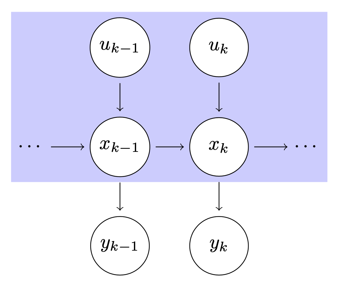
\begin { pgfonlayer}{ background}
\fill [blue!20!white] (strect start) rectangle (strect end);
\end { pgfonlayer}
\end { tikzpicture}
囲み枠(Fitting Library利用)# 参考 PGF Manual, Part V, 54 Fitting Library
前節では、青色の四角形の座標を\coordinate (strect start) ...と\coordinate (strect end) ...で計算している。このケースではそこまで複雑ではないが、ノードの囲み枠の座標を計算せずに描画したいなら、Fittingライブラリが使える。
\node [fit=...] {};で囲み枠を作成。...の部分にはスペース区切りのノードが入る。枠の余白を調整したいならinner sepを指定する。
1
2
3
4
5
6
7
8
9
10
11
12
13
14
15
16
17
18
19
20
21
22
23
24
25
26
27
28
29
30
31
32
33
34
35
36
37
\usetikzlibrary { positioning, graphs, fit}
\pgfdeclarelayer { background}
\pgfsetlayers { background, main}
\begin { tikzpicture}
\matrix [row sep=2em, column sep=2em,
entity/.style={ draw, circle,
minimum width=3em,
outer sep=3pt,
fill=white} ] {
\coordinate (instart) at (0,0);
& \node [entity] (in0) { $ u_{k - 1 } $ } ;
& \node [entity] (in1) { $ u_{k} $ } ;
& \\
\node [] (ststart) { $ \cdots $ } ;
& \node [entity] (st0) { $ x_{k - 1 } $ } ;
& \node [entity] (st1) { $ x_{k} $ } ;
& \node [] (stend) { $ \cdots $ } ;\\
& \node [entity] (ob0) { $ y_{k - 1 } $ } ;
& \node [entity] (ob1) { $ y_{k} $ } ;
& \coordinate (obend) at (0,0); \\
} ;
\graph {
(ststart) -> (st0) -> (st1) -> (stend);
(in0) -> (st0) -> (ob0);
(in1) -> (st1) -> (ob1);
} ;
\begin { pgfonlayer}{ background}
\node [fit=(in0) (in1) (ststart) (st0) (st1) (stend),
fill=blue!20!white,
inner sep=0pt] {} ;
\end { pgfonlayer}
\end { tikzpicture}
結果の画像は前節と同様なので省略。
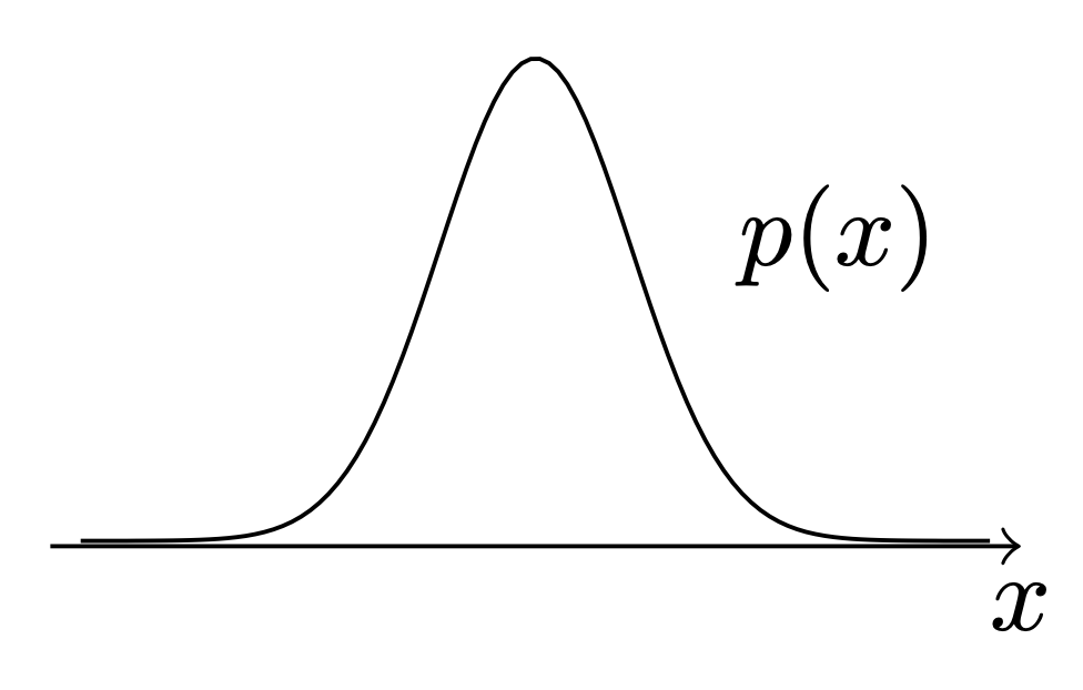
関数のグラフの描画# 参考 PGF Manual, Part III, 22.5 Plotting a Function
簡単な関数の描画ならplotを使う。
plotは\drawコマンドの中で指定できる。基本的にはplot (\x, {\xについての関数})のような形で書く。domainで定義域、samplesでサンプル数(大きいほど滑らか)を指定。
\x^2ではなく(\x)^2としないと2乗が正しく計算されないことに注意。
1
2
3
4
5
\begin { tikzpicture}
\draw [domain=-1.5:1.5, samples=100] plot (\x , { exp(-(\x )^ 2/(2*0.1))/(2*pi*0.1)} );
\draw [->, yshift=-0.5pt] (-1.6,0) -- (1.6,0) node [below] { $ x $ } ;
\node at (1, 1) { $ p ( x ) $ } ;
\end { tikzpicture}
あまり複雑な関数だとTeXでは効率的に計算できないらしいので、その場合はgnuplotと連携する方法を検討したほうが良いらしい(参考:PGF Manual, Part III, 22.6 Plotting a Function Using Gnuplot)。
gnuplotで連携する以外にも、pyplotなど外部プログラムで予め画像を作っておき、それを\includegraphicsで読み込む方法が考えられる。実際、TikZでは以下のようにnodeの中に画像を埋め込める。
1
\node at (0,0) { \includegraphics [width=1cm, clip] { path/to/file.pdf}} ;
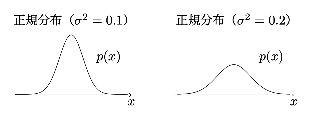
座標を使った平行移動# xshiftで横軸方向、yshiftで縦軸方向の平行移動が可能。
それだけでなく、shift={(座標)}で縦軸、横軸まとめて平行移動が可能。
 1
 2
 3
 4
 5
 6
 7
 8
 9
10
11
12
13
14
15
16
17
18
19
20
\usetikzlibrary { calc, positioning}
\begin { tikzpicture}
\node (a) { 正規分布($ \sigma ^ 2 = 0 . 1 $ )} ;
\node [right=1cm of a] (b) { 正規分布($ \sigma ^ 2 = 0 . 2 $ )} ;
\begin { scope} [shift={ ($ ( a.south ) + ( 0 , - 1 . 7 cm ) $ )} ]
\draw [domain=-1.5:1.5,
samples=100] plot (\x , { exp(-(\x )^ 2/(2*0.1))/(2*pi*0.1)} );
\draw [->, yshift=-0.5pt] (-1.6,0) -- (1.6,0) node [below] { $ x $ } ;
\node at (1, 1) { $ p ( x ) $ } ;
\end { scope}
\begin { scope} [shift={ ($ ( b.south ) + ( 0 , - 1 . 7 cm ) $ )} ]
\draw [domain=-1.5:1.5,
samples=100] plot (\x , { exp(-(\x )^ 2/(2*0.2))/(2*pi*0.2)} );
\draw [->, yshift=-0.5pt] (-1.6,0) -- (1.6,0) node [below] { $ x $ } ;
\node at (1, 1) { $ p ( x ) $ } ;
\end { scope}
\end { tikzpicture}
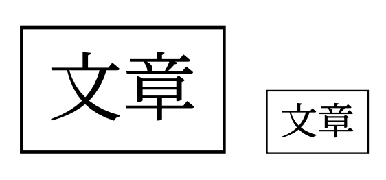
図を拡大縮小する(TikZの話ではない)# 図がPDFの文書からはみ出たり、逆に小さすぎたりした場合、位置やフォント、図形のサイズをうまく調整して直すべきではあるのだが、それでも難しい場合の最終手段として「tikzpicture環境内の図形をまるごと拡大縮小する」がある。それには\scaleboxコマンドを使う。これはTikZではなく、LaTeXのコマンドである(参考:LaTeX2e unofficial reference manual 22.3.3 )。以下のように、環境全体をくくって使う。
1
2
3
4
5
6
7
8
\begin { tikzpicture}
\node [draw] { 文章} ;
\end { tikzpicture}
\scalebox { 0.5}{
\begin { tikzpicture}
\node [draw] { 文章} ;
\end { tikzpicture}
}
拡大縮小しすぎて図が見づらくなる危険があるため、むやみな使用は禁物かもしれない。
(補足 \begin{tikzpicture}[scale=0.5]...のようにscaleを指定しても縮小可能なのではないか、と感じるが、実際は期待通りにはならない。このscaleは座標系の縮尺を変更するだけで、図形やテキストのサイズには変化を及ぼさない。)
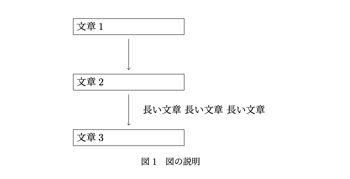
特定の座標を中心にした水平方向の中央寄せ# 以下のようにfigure環境でくくり、\centeringを使って中央寄せしたケースを考える。
 1
 2
 3
 4
 5
 6
 7
 8
 9
10
11
12
13
14
15
16
17
18
\begin { figure}
\centering
\begin { tikzpicture} [
node/.style={ draw, minimum width=10em, text width=10em, outer sep=4pt, align=left} ,
]
\node [node] (a) {
\begin { minipage}{ \linewidth }
Step1
\par { \centering 文章1}
\end { minipage}} ;
\node [node, below=3em of a] (b) { 文章2} ;
\node [node, below=3em of b] (c) { 文章3} ;
\draw [->] (a) -- (b);
\draw [->] (b) -- node[right=1em] { 長い文章 長い文章 長い文章} (c);
\end { tikzpicture}
\caption { 図の説明}
\end { figure}
結果は以下のようになる。
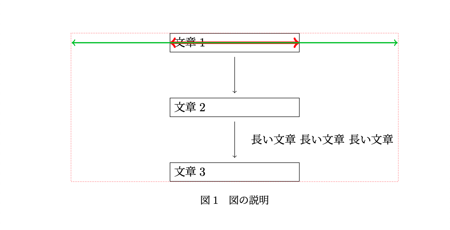
ここで、「文章1」「文章2」「文章3」のノードが、水平方向に対し中央に来るように中央寄せしたい。
調べてみたところ,2つの方法があった.
use as bounding boxを利用した方法(参考 )pathコマンドで左右を引き伸ばす(参考 )個人的には後者がクセが無くて使いやすいので,後者の方法のみ記す.
あるノードを視点として、左右対称に線を引けば良い。そうすれば勝手にbounding boxが伸び、中央寄せになる。
1
2
3
4
5
6
7
8
9
10
11
12
13
14
15
16
17
18
19
20
21
22
23
24
\begin { figure}
\centering
\begin { tikzpicture} [
node/.style={ draw, minimum width=10em, text width=10em, outer sep=4pt, align=left} ,
]
\node [node] (a) { 文章1} ;
\node [node, below=3em of a] (b) { 文章2} ;
\node [node, below=3em of b] (c) { 文章3} ;
\draw [->] (a) -- (b);
\draw [->] (b) -- node[right=1em] { 長い文章 長い文章 長い文章} (c);
\draw [<->, red, line width=2pt]
($ ( current bounding box.west | - a ) $ ) --
++ ($ - 2 *( $ (current bounding box.west |- a) - (a)$ ) $ );
\draw [<->, green!75!black, line width=1pt]
($ ( current bounding box.east | - a ) $ ) --
++ ($ - 2 *( $ (current bounding box.east |- a) - (a)$ ) $ );
\draw [densely dotted, red]
(current bounding box.north west) rectangle (current bounding box.south east);
\end { tikzpicture}
\caption { 図の説明}
\end { figure}
上記のコードは、bounding boxの広がりを矢印で可視化するために冗長に書いてある。
よりシンプルで、かつ矢印や点線を書かないなら、以下のようにする。
1
2
3
4
5
6
7
8
9
10
11
12
13
14
15
16
17
\begin { figure}
\centering
\begin { tikzpicture} [
node/.style={ draw, minimum width=10em, text width=10em, outer sep=4pt, align=left} ,
]
\node [node] (a) { 文章1} ;
\node [node, below=3em of a] (b) { 文章2} ;
\node [node, below=3em of b] (c) { 文章3} ;
\draw [->] (a) -- (b);
\draw [->] (b) -- node[right=1em] { 長い文章 長い文章 長い文章} (c);
\path (a) -- ++($ - 1 *( $ (current bounding box.west |- a) - (a)$ ) $ )
(a) -- ++($ - 1 *( $ (current bounding box.east |- a) - (a)$ ) $ );
\end { tikzpicture}
\caption { 図の説明}
\end { figure}
この方法はHow to center horizontally tikzpicture in beamer frame using a specific node?- Stack Exchange を参考にした。こちらでは「ベクトルを-1倍する」という操作を「180度回転させる」という操作にしてコードを書いているようだ。
参考サイトのように、\tikzsetを使って再利用したい場合は次にようにする(プリアンブルに書いておく)。
1
2
3
4
5
6
7
8
\tikzset {
center coordinate/.style={
execute at end picture={
\path (#1) -- ++($ - 1 *( $ (current bounding box.west |- #1) - (#1)$ ) $ )
(#1) -- ++($ - 1 *( $ (current bounding box.east |- #1) - (#1)$ ) $ );
}
}
}
これは以下のように、center coordinate=aのように使う。
1
2
3
4
5
6
7
8
9
10
11
12
13
14
15
\begin { figure}
\centering
\begin { tikzpicture} [
center coordinate=a,
node/.style={ draw, minimum width=10em, text width=10em, outer sep=4pt, align=left} ,
]
\node [node] (a) { 文章1} ;
\node [node, below=3em of a] (b) { 文章2} ;
\node [node, below=3em of b] (c) { 文章3} ;
\draw [->] (a) -- (b);
\draw [->] (b) -- node[right=1em] { 長い文章 長い文章 長い文章} (c);
\end { tikzpicture}
\caption { 図の説明}
\end { figure}
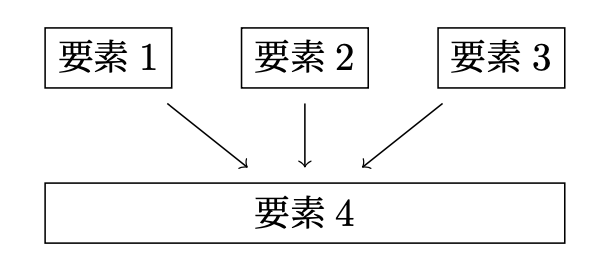
ノードの幅や高さを合わせる# 他にもあるかもしれないが,頑張って幅を計算する方法と、Fittingライブラリを使う方法の2種類が考えられる.
(方法1)letを使って幅を計算する# こちらは自分で考えた方法.
以下のように、letを使って |(a.westのx座標) - (c.eastのy座標)| を計算し、それをminimum widthに設定する。ただし、a.westとc.eastの座標はouter sepに影響を受けるため、その分を差し引きする。
1
2
3
4
5
6
7
8
9
10
11
12
13
14
15
16
17
18
19
\begin { tikzpicture} [
node/.style={ draw, outer sep=4pt} ,
]
\node [node] (a) { 要素1} ;
\node [node, right=1em of a] (b) { 要素2} ;
\node [node, right=1em of b] (c) { 要素3} ;
\coordinate (d) at ($ ( a )! 0 . 5 !( c ) + ( 0 , - 4 em ) $ );
\path let \p 0 = (a.west),
\p 1 = (c.east),
in
node [node, minimum width={ abs(\x 1-\x 0) - 2*4pt} ]
(d) at ($ ( a )! 0 . 5 !( c ) + ( 0 , - 4 em ) $ ) { 要素4} ;
\draw [->] ($ ( a.south west )! 0 . 5 !( c.south east ) $ ) -- (d);
\draw [->] ($ ( a.south west )! 0 . 25 !( c.south east ) $ ) -- (d);
\draw [->] ($ ( a.south west )! 0 . 75 !( c.south east ) $ ) -- (d);
\end { tikzpicture}
(方法2)Fitting Libraryを使う# 参考 Creating a node fitting the horizontal width of two other nodes
以下のように、fit={(a) (b) (c)}を\nodeのオプションとして指定すれば、
(a) (b) (c)を囲むノードが作成できる。これをyshiftを使い下にずらす。
テキストはlabelオプションで指定している。
1
2
3
4
5
6
7
8
9
10
11
12
13
\begin { tikzpicture} [
node/.style={ draw, outer sep=4pt} ,
]
\node [node] (a) { 要素1} ;
\node [node, right=1em of a] (b) { 要素2} ;
\node [node, right=1em of b] (c) { 要素3} ;
\node [node, fit={ (a) (b) (c)} , inner sep=-4pt, label={ center:要素4} , yshift=-4em] (d) {} ;
\draw [->] ($ ( a.south west )! 0 . 5 !( c.south east ) $ ) -- (d);
\draw [->] ($ ( a.south west )! 0 . 25 !( c.south east ) $ ) -- (d);
\draw [->] ($ ( a.south west )! 0 . 75 !( c.south east ) $ ) -- (d);
\end { tikzpicture}
(補足)ノードのテキストについて# ノードのテキストを\node [...] (d) {...}の{...}の部分に指定すると、若干上にずれる
(Fittingライブラリの仕様のようだが、なぜそのようなことが起こるのかは良くわかっていない)。
“PGF Manual Part V, 54 Fitting Library"の/tikz/every fitの説明の下に書かれている文章によると、
(中略) The above means that, generally speaking, if the node contains text like box in the above example, it will be centered inside the box. It will be difficult to put the text elsewhere, in particular, changing the anchor of the node will not have the desired effect. Instead, what you should do is to create a node with the fit option that does not contain any text, give it a name, and then use normal nodes to add text at the desired positions. Alternatively, consider using the label or pin options.
とある。別の\nodeを作成してそこにテキストを書いたり、labelやpinオプションを使ってテキストを指定したりすると良いらしい。